M3d Finite Element Local Coordinates TutoriaL
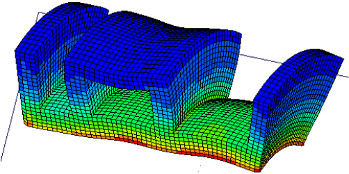
This page gives a demonstration of how to use the newly added local coordinate systems to model a component with sectorial symmetry

First we need to create a simple model. In M3d select the 'Rectangle Icon' illustrated left.
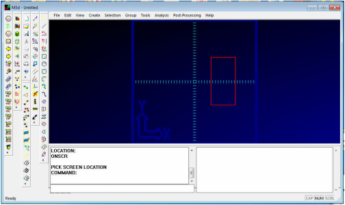
Click two points on the screen to define a rectangle. Pick the top left corner and then the bottom right in the approximate locations shown.

Now we will loft a surface between both vertical lines of the rectangle. Select the icon displayed left

You will then be prompted to pick the cross-section curves. Select the two vertical lines from the screen and press enter or click the middle mouse button. Press the 'Shaded Display button illustrated left.
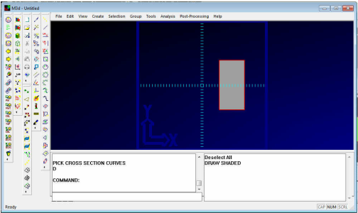
The surface should appear as shown right. Note the two cross-section curves will still appear highlighted as they are still in the selection buffer. To deselect the curves, from the right mouse button menu select the 'Deselect All' menu item.

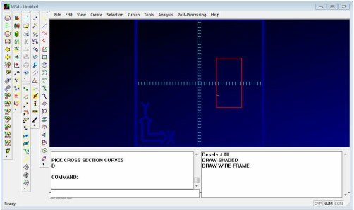
To return to wire frame display select the icon shown left.
Note the U marker on the surface indicating the surfaces U parametric direction.

Now we will create a mapped mesh on the surface by selecting the 'Mapped Quad Mesh on Surface' Icon illustrated left. Note this does not work with trimmed surface presently.
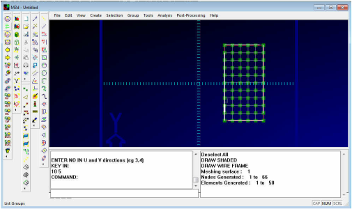
You will then be prompted to pick the surface. Select the surface from the screen then press enter, or double click the middle mouse button or "done". Then enter the number of elements required in the surface U and V directions by typing 10,5 in the command line. The Finite Element quad mesh should be generated as shown opposite.

We now need to align the work plain in an orientation with Z where the Y is currently. This is so we can sweep the shell elements into solid elements around the work plain Z-axis with the work plain in cylindrical mode. To do this, we will first create a line in the current Y direction and then we align the work plain to this. To create the line select the 'Line' icon shown left
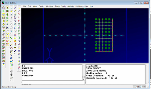
You are then prompted for two points, in the command line type '0,0,0' then press enter. Then type '0,1,0' in the command line for the second point. The line should have been created as illustrated opposite
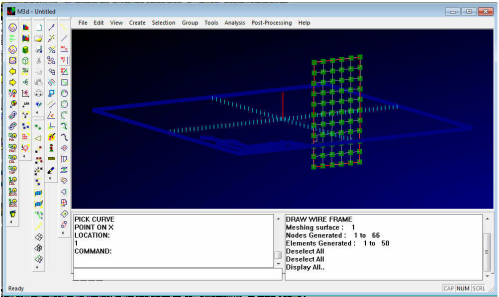
From the main menu select 'Tools->Workplain->WP Align to Curve'. You are then prompted to pick a curve to align the workplain to. This will align the work plains Z-axis to the curves' direction. Pick the newly created curve. Then you will be asked to pick a point to define the work plains' X direction, type '1,0,0' in the command line. The work plain should now be positioned as shown opposite.
Note: Pressing F1 and moving the mouse pans the display, F2 zooms and F3 rotates
Note: Pressing F1 and moving the mouse pans the display, F2 zooms and F3 rotates
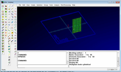
We now need to toggle the work plain into cylindrical mode. Select 'Tools->Workplain->WP Mode' from the main menu. The X and Y work plain axis markers should have been replaced with R and Theta. Now all operations will be based on a cylindrical coordinate system
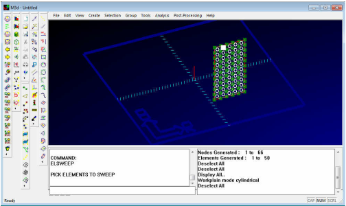
We are now going to sweep the shell elements (in a cylindrical system) into solid brick elements. From the main menu select 'Create->Mesh->Sweep Elements'. You are then prompted to pick the elements to sweep. Drag a box over the elements by pressing down the left mouse button and dragging the mouse to right and down. When the left button is released the elements should be selected as illustrated opposite
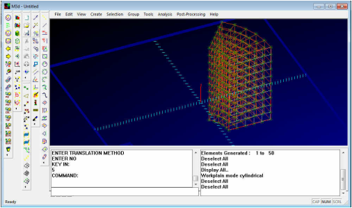
Pressing enter or clicking the middle mouse button accepts this selection. You are then prompted for a translation method. This can be either 'Key In' or 'Pick'. the 'Key In' method requires you to type the translation vector into the command line. The 'Pick' method gets the translation vector by asking you to select two items from the screen. From the right mouse button menu select 'Key In'. In the command line type 0,10 (which means translate by 10 degrees in the work plain cylindrical system) then press enter. You are then asked for the number of copies, e.g. for this example we have typed '5' in the command line. The solid elements shown opposite should have been generated.

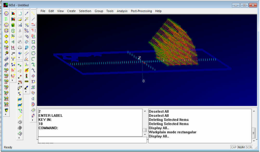
Note the shell elements are still highlighted as we don't want these press the 'delete icon' shown left.
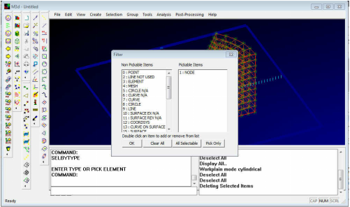
The nodes that were on the shell elements now still exist as free nodes which we will now delete. To make sure we pick only the nodes from the right mouse button menu select 'Filter'. This brings up the filter dialog box which determines which items are selectable from the screen. From this select 'NODE' from the list and press the 'Pick Only' button.

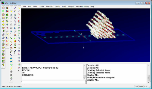
With the filter set it is only possible to pick nodes. Drag a box over the entire model and press the 'delete icon' shown left, note: only free nodes will be deleted. Select the filter again, from the right mouse button menu, and make everything selectable again.
Note the commands set the filter depending on what they are expecting you to pick. Sometimes they don't set it back to 'All'. If you encounter problems selecting items - check the filter.
Note the commands set the filter depending on what they are expecting you to pick. Sometimes they don't set it back to 'All'. If you encounter problems selecting items - check the filter.
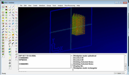
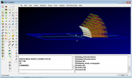
Now set the work plain back to its global position by selecting 'Tools->Workplain->WP to Global' from the main menu and back to Cartesian with 'Tools->Workplain->WP Mode

Now we need to create a local cylindrical coordinate system for the nodal degrees of freedom to reference. From the tool bar select the 'Create Coordinate System icon shown right.
You are then prompted for the coordinate systems center point (origin) location. In the command line type 0,0,0 and press enter. Now we are asked for a point on the coordinate systems X-axis. In the command line type 1,0,0 and press enter and then supply a point on the XY plain (e.g. type 0,0,1). To finish enter '2' for the coordinate systems type (in this example, cylindrical) and '10' for the ID. The coordinate system should have been created as shown opposite.
The nodal output coordinate system now needs to be modified to reference coordinate system 10. From the main menu select 'Tools->Node Modify->Output Coordinate System'. Select all the nodes by dragging a box over them and then press enter or click the middle mouse button. Then as prompted enter '10' as the new nodal output coordinate system. Now, when forces and restraints are applied to the model they will be in the coordinate system 10 directions.
Now is a good time to remove the surface we created from the display. From the main menu select 'View->Visablity->Surface->Surfaces On/Off' this toggles their visibility.
We are now going to create radial forces on the inner surface of the mesh. First we shall pre-select the nodes before entering the command.
Rotate the model (F2 button and mouse move) until looking down on top as illustrated opposite. Drag a box over the nodes on the inner edge to select them.
Note the nodes have been selected even though not in a command. If you can't select the nodes check the filter under the right mouse button menu and make sure nodes are selectable.
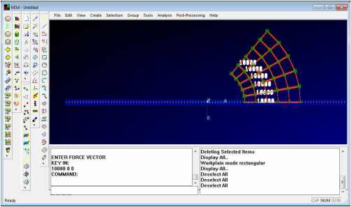
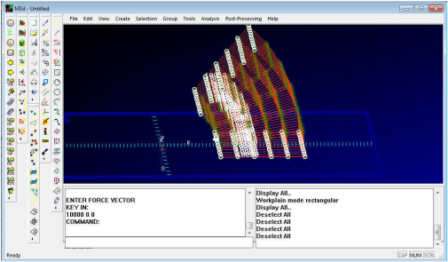
From the main menu select 'Analysis->Create Force'. You are then prompted to pick the nodes. As they are already selected, press enter or click the middle mouse button. Then as prompted enter the force vector 10000,0,0 in the command line and press enter.
The forces should be created as illustrated opposite. Note the force directions are in the radial coordinate system 10 direction
The forces should be created as illustrated opposite. Note the force directions are in the radial coordinate system 10 direction
We now need to create theta restraints along the symmetry plains. Select the nodes along the plains as illustrated opposite.
Remember if you want to avoid picking elements accidentally, set the filter to pick 'nodes only'.
Remember if you want to avoid picking elements accidentally, set the filter to pick 'nodes only'.
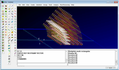
From the main menu select 'Analysis->Create Restraint' you are then prompted for the nodes, as they are pre-selected, press enter. You are then prompted for the translational restraint vector. Type 0,1,0 and press enter and 0,0,0 for the rotational restraints. The two symmetry plains are now restrained in the theta direction.
An '0' in the vector string means no restraint and '1' means restrain.
An '0' in the vector string means no restraint and '1' means restrain.
In a similar manner create some Z restraints on the bottom surface. The restraint vectors being 0,0,1 and 0,0,0
To create a material for these elements select: 'Create->Material->Isentropic' from the main menu.
You will then be prompted for a:
Title - Give it a name
MID - Accept the default or enter a unique ID (1)
E - Young modulus (210e9 for our example)
V - poisons ratio (0.29)
Density - optional for linear statics
CTE - Co-efficient of thermal expansion
Now the material is defined, we can create the property for the solid finite elements.
From the main menu select: 'Create->Property->Solid'
You will then be prompted for a:
Title - Give it a name
PID - Accept the default or enter a unique ID (1)
MID - Enter the material ID as specified for the material (1)
We now need to update our solid elements with this new property.
From the main menu select: 'Tools->Element Modify->PID'. You are then prompted to pick the elements to update. Select all the element by dragging a box over them and press enter or click the middle mouse button. Then enter '1' for the new PID as created above.
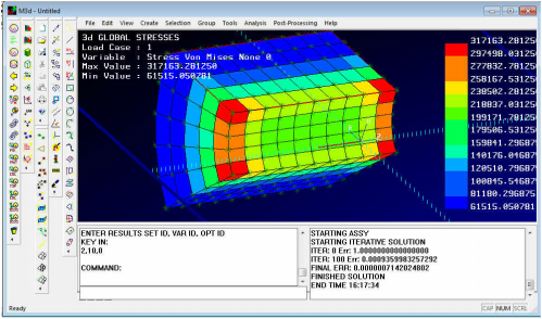
Now we can solve the model from the main menu. Select 'Analysis->Solve Stress'
Note: The new local coordinate systems have just been added to the solver. They use a large stiffness value transformed to the restraint directions to enforce the restraint. This large stiffness has the effect of making the iterative solver slower to converge. We are still evaluating what is the most appropriate value to use.
Note: The new local coordinate systems have just been added to the solver. They use a large stiffness value transformed to the restraint directions to enforce the restraint. This large stiffness has the effect of making the iterative solver slower to converge. We are still evaluating what is the most appropriate value to use.