Creating a basic thermal model
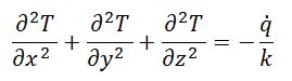
This page is intended to give a guide to creating a basic thermal model which solves the steady state Poisson's equation with heat generation as shown below.
The thermal model at present only supports heat sources and sinks and the application of boundary temperatures. Convective wall functions and radiant heat exchange will be added shortly.
The thermal model at present only supports heat sources and sinks and the application of boundary temperatures. Convective wall functions and radiant heat exchange will be added shortly.
This also serves as a good tutorial in understanding how to create F.E. models in M3d. There have been a lot of changes to this version which need explanation.
The process of creating an F.E. model in M3d (short version).
1) Create the model - nodes and elements
2) Create a material property
3) Create properties for each different element group
4) Assign the properties to the groups of elements
5) Perform checks
Coincident nodes
Free edge
Free face
6) Create load and boundary sets
7) Apply loads and boundary conditions
8) Create a solution
Linear static or
Steady state thermal
9) Create a solution step (basically a subcase)
10) Activate the step to be solved
11) SOLVE
12) Post-process results
Creating a NEW MODEL
Open M3d and save the empty model to a name of your choice. I recommend that you save M3d before any significant operation as there is no undo and we still have bug issues.
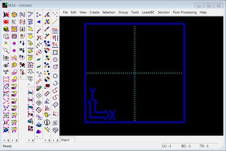
The open session should appear as shown opposite. The work-plane is clearly shown in blue. All coordinates and operations in M3d are relative to the work-plane , the work-plane can be moved, re-oriented and re-sized to aid with modelling.
The open session should appear as shown opposite. The work-plane is clearly shown in blue. All coordinates and operations in M3d are relative to the work-plane , the work-plane can be moved, re-oriented and re-sized to aid with modelling.
Creating a rectangle
We are going to create a rectangular surface which we will mesh with quad elements. These elements will then be extruded into brick elements to create a solid bar.

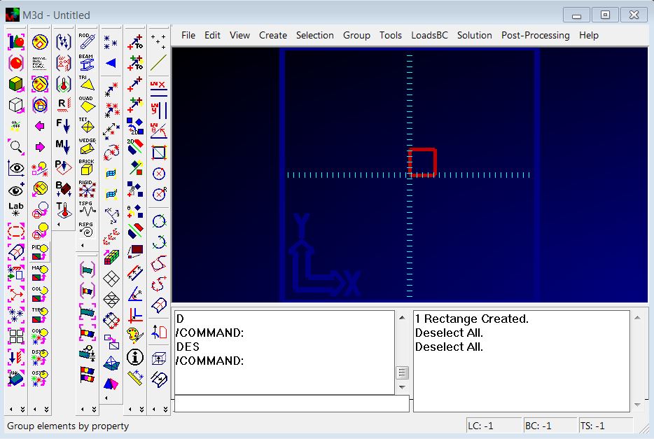
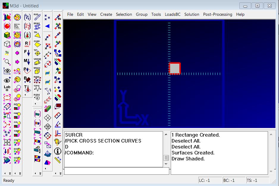
Select the create rectangle icon shown left (or menu item Create->Rectangle). You will be prompted for the two corners defining the bottom left and top right corners of the rectangle. In the command window type 0,0 and press enter for the first point then 0,1 for the second and then enter. A unit rectangle should be created on the screen as shown below.
Creating a lofted surface

To create a lofted surface click the surface create icon shown left (or Create->Surface->Loft from the menu). Now pick two opposite edges of the rectangle from the screen and press enter.

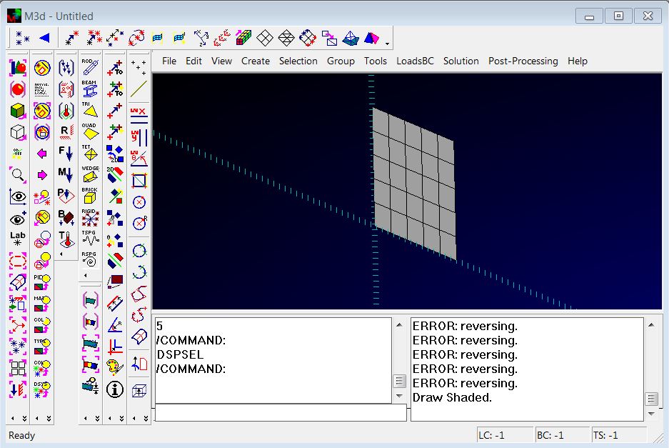
A lofted surface should now have been created. To view the model in shaded mode click the shaded view icon shown left (or select the View->Shaded menu item.)
The shaded view is shown below.
The shaded view is shown below.
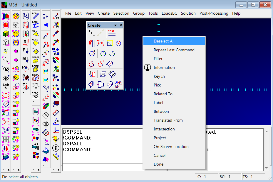
Note the two edges of the rectangle are still highlighted, meaning they are still in the selection buffer. To clear the selection buffer right click the mouse in the viewing window and select "Deselect All" from the mouse menu as illustrated below.

To return the view to wireframe mode click the icon shown left (or select View->Line from the menu).
Creating a mapped quad mesh

To create a mapped quad mesh on the newly created surface pick the icon shown opposite (or select Create->Mesh->Mapped QUAD mesh. from the menu)
Pick the surface from the screen and select "Done" from the right mouse menu (or press Enter).
Now in the command line enter the number of elements to create in both the surface u & v directions. Type 5,5 and press enter. The mesh on the surface should now have been created as illustrated below.
Pick the surface from the screen and select "Done" from the right mouse menu (or press Enter).
Now in the command line enter the number of elements to create in both the surface u & v directions. Type 5,5 and press enter. The mesh on the surface should now have been created as illustrated below.

DYNAMIC VIEWING.
To zoom in/out of the view scroll the mouse wheel.
To pan the model left-right up-down hold down the middle mouse button and move the mouse.
To rotate the model hold down the shift key and move the mouse in the viewing window.
Alternatively you can press down F1, F2 or F3 and move the mouse.
To pan the model left-right up-down hold down the middle mouse button and move the mouse.
To rotate the model hold down the shift key and move the mouse in the viewing window.
Alternatively you can press down F1, F2 or F3 and move the mouse.
Free edge display
To display the free edges of the mesh, as a check, select the "Tools->Checks->Free Edge Display" menu item. Then on the screen drag a box (from top left to bottom right) over all the elements and select "Done" from the right mouse menu or press enter. The model should now appear as illustrated below with the edges highlighted. This is an important check in F.E. for mesh continuity and cracks will become evident.
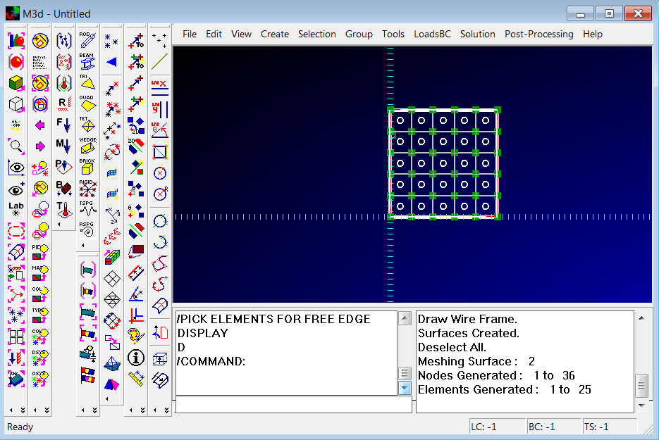
Note the elements appear highlighted with a circle at their centroid - remember to clear them from the selection buffer by selecting "Deselect All" from the right mouse menu. If you don't do this they may get inadvertently used in your next operation. In this case they will be used for the next command.
sweeping shells to solid elements

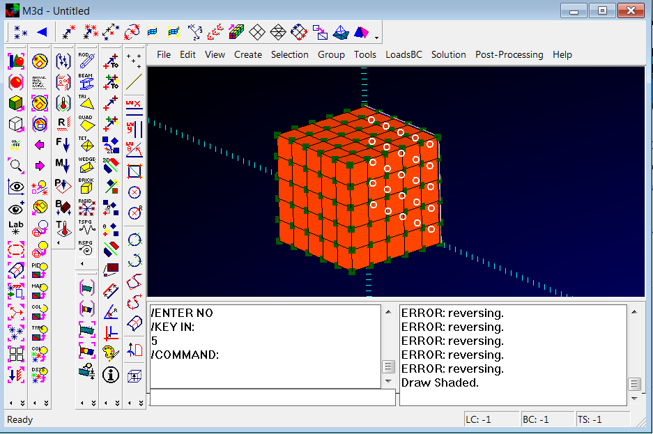
To sweep the shell elements into solids select the icon shown left (or select Create->Mesh->Sweep Elements from the menu). You then need to select the elements to sweep. If they are not selected drag a box over the elements on the screen or pick them individually. When they are selected press enter or select "Done" from the right mouse menu.
You will then be prompted for the translation method.
/ENTER TRANSLATION METHOD (PICK or KEY)
The "PICK" method means a vector will be defined by selecting two objects from the screen. The "KEY" method will expect you to enter a vector into the command line. In this case we will "KEY" in the vector. To select this option either type "KEY" into the command line or select "Key In" from the right mouse menu.
In the command line type the vector "0,0,0.2" and press enter. You will then be prompted for the number of copies, type 5 for this and enter. The model illustrated below should have been created.
DISPLAY SELECTED

You will notice the shell elements used for this operation are still highlighted. To illustrate another important feature of M3d - to isolate the selected items in the display you can press the "Display Selected" icon shown left (or select "View->Display Selected menu item). The result is illustrated below and this feature is extremely useful for reducing the number of items on the screen when working on a model.
DISPLAY ALL

To display the whole model again click the icon shown left (or select View->Display All menu item).
DELETE

These elements are not needed and must be deleted. If they are not still selected then drag a box over them to re-select and click the Trash Can icon shown left.
FILter
Note also that some nodes related to the shell elements still exist and are not connected to the solid elements. These need to be deleted too. This will illustrate another important concept in M3d for selecting items of a particular type - the Filter.
From the right mouse button menu select the option "Filter" this will display the Selection Filter dialog box as illustrated below.
From the right mouse button menu select the option "Filter" this will display the Selection Filter dialog box as illustrated below.
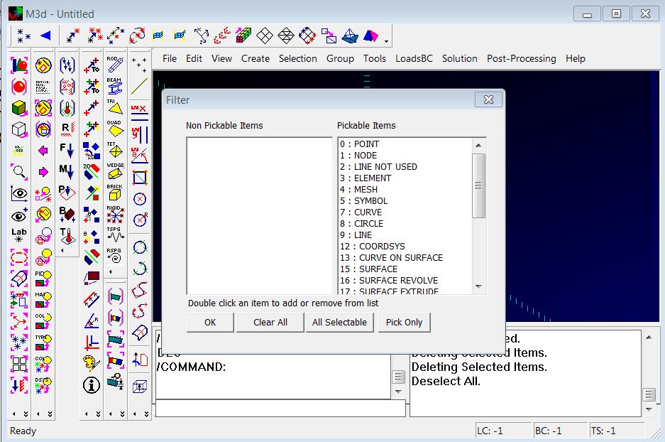
In the dialog box pick node from the list and click the "Pick Only" button. This makes only nodes pick-able. Drag a box over the entire model, now only the nodes should be selected as illustrated below.
Once more, click the delete Trash Can icon to delete the selected nodes. Note only free nodes will be deleted. It is good practice to do this process of deleting all the nodes in any model before going further.
Now bring up the Filter dialog box once more and click the "All Selectable" button and "Ok". This resets everything to be selectable.
Now bring up the Filter dialog box once more and click the "All Selectable" button and "Ok". This resets everything to be selectable.
DEFINING A MATERIAL
From the menu select "Create->Material->Isentric" and enter the following in the command line as prompted.
/ENTER MATERIAL TITLE
AL
/ENTER NEW MID (1)
1
/ENTER E
70E9
/ENTER V
0.33
/ENTER DENSITY
2750
/ENTER CTE
23E-6
/ENTER THERMAL CONDUCTIVITY k
200
This will create a property for Aluminium with an ID of 1.
/ENTER MATERIAL TITLE
AL
/ENTER NEW MID (1)
1
/ENTER E
70E9
/ENTER V
0.33
/ENTER DENSITY
2750
/ENTER CTE
23E-6
/ENTER THERMAL CONDUCTIVITY k
200
This will create a property for Aluminium with an ID of 1.
DEFINING A PROPERTY For the solid elements
To create a property for the solid elements from the main menu select "Create->Property->Solid" and follow the prompts in the command window as shown below. Comments are added proceeded by <-.
PRSOLID
/ENTER PROPERTY TITLE
SOLID ELEMENTS <- Enter property title
ENTER NEW PID (1)
1 <- Enter the property ID
/ENTER MID
1 <-The ID of the material we just created
PRSOLID
/ENTER PROPERTY TITLE
SOLID ELEMENTS <- Enter property title
ENTER NEW PID (1)
1 <- Enter the property ID
/ENTER MID
1 <-The ID of the material we just created
Scripting
Note M3d supports a basic form of scripting for most commands. If you were to cut and paste the above lines (minus the comments) into to the command line the commands would be executed.
Assigning the property to the elements
From the menu select the Tools->Element Modify->Property ID (PID) you will then be prompted to pick the elements to modify. Drag a box over all the elements and from the right mouse menu select "Done" or press enter. In the command window enter 1 for the new property ID for the elements to reference and enter. From the right mouse menu select "Deselect All" to clear the elements from the selection buffer.
Create A LOAD SET

We now need to create a loadset to contain our flux loading for the solve. You can create as many loadsets as you like which can be assigned to different subcases (steps) in the solution.
Loads that you create go automatically into the active loadset, so be careful the correct loadset is active when you create loads for that particular case.
From the menu select "LoadsBC->Load Sets" or click the icon shown left. This will bring up the loadsets dialog box show below.
Loads that you create go automatically into the active loadset, so be careful the correct loadset is active when you create loads for that particular case.
From the menu select "LoadsBC->Load Sets" or click the icon shown left. This will bring up the loadsets dialog box show below.
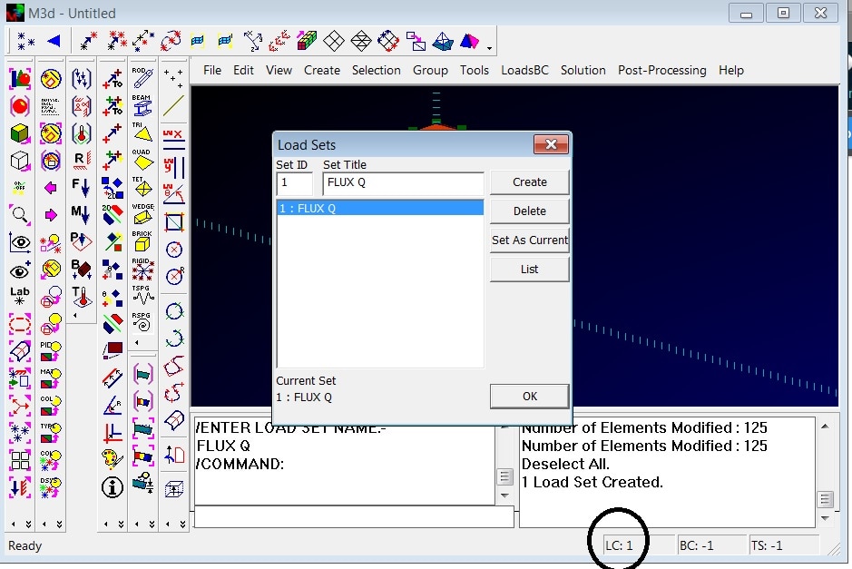
Enter an ID for the loadset and a title as shown above. Press the "Create" button to create the loadset and then the "Set as Current" button to make it the active set. Notice the status line indicator which displays the ID of the active loadset. All loads created from now on will go into this set until it is changed.
Creatre a boundary SET

In a similar way we need to create a boundary set to contain the boundary conditions in the model. These will be fixed boundary interface temperatures.
From the menu select "LoadsBC->BC Sets" or click the icon shown left. Create the set as illustrated below and set it as active.
From the menu select "LoadsBC->BC Sets" or click the icon shown left. Create the set as illustrated below and set it as active.
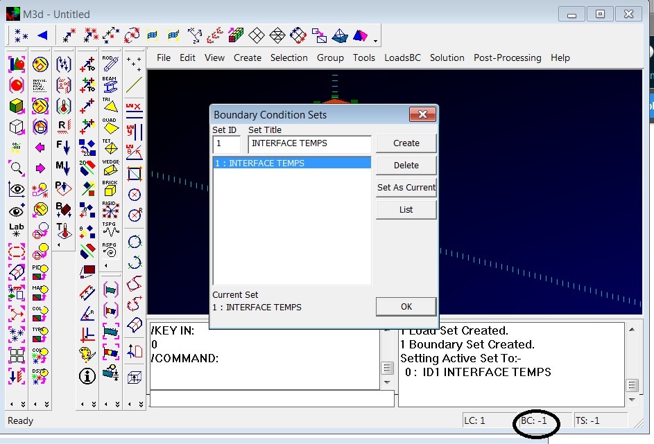
CREATING A BOUNDARY TEMPERATURE
We now need to create a fixed boundary temperature on one face of our model. Note for most of the thermal models at least one boundary temperature is required.
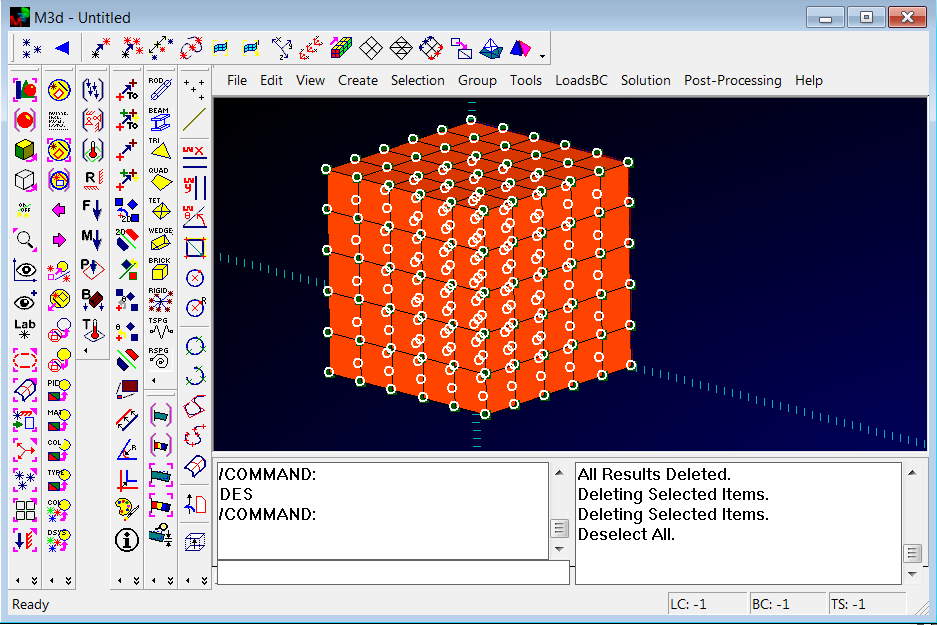
From the menu select LoadsBC->Create Thermal Temp BC. Orientate the model and select the nodes as illustrated below and then press enter or "Done".
From the menu select LoadsBC->Create Thermal Temp BC. Orientate the model and select the nodes as illustrated below and then press enter or "Done".
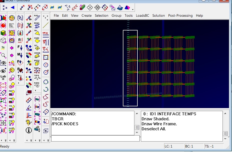
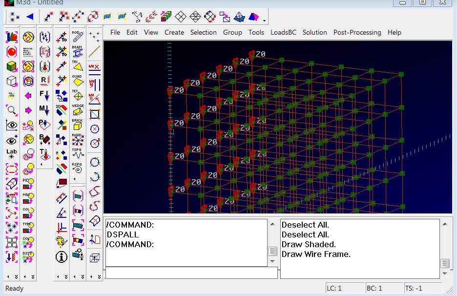
Enter a value of 20 in the command window for the Temperature and enter. The model should now appear as below with temperature markers on the selected face.
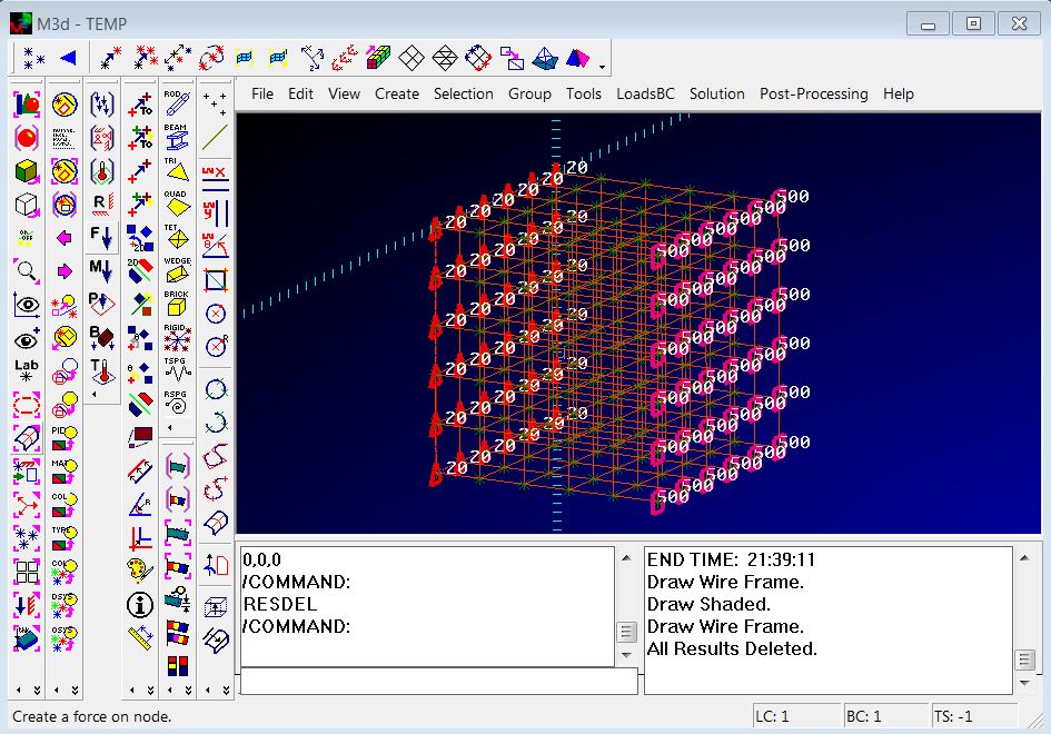
Creating a flux heat source
We will now repeat this process but creating a heat flux source on the opposite face. From the menu select "LoadsBC->Create Thermal Nett Flux Load" select the nodes on the opposite face and enter 500 for the flux value. The model should appear as shown below.
CREATING A SOLUTION
We now need to define a solution sequence for the solver. From the menu select "Solution->Create Solution" this invokes the solutions dialog box as as illustrated below.
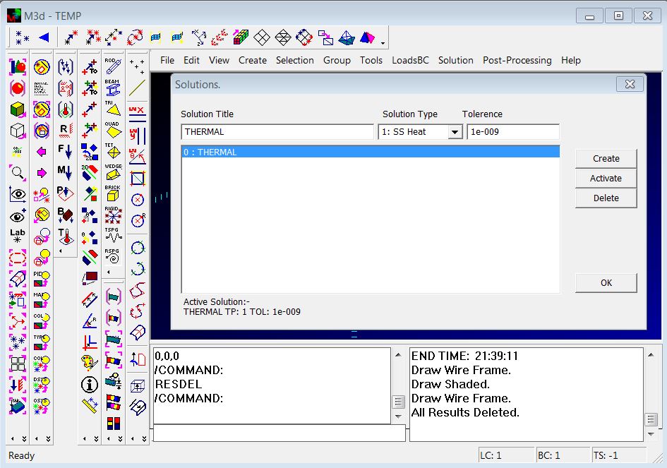
Enter a title for the solve and select "SS Heat" as the solution type. The tolerance is the ratio of change in the solution results from one iteration to the next 1e-9 is extremely accurate and can be reduced to speed up solutions. This needs to be done with consideration of accuracy to speed, but as the solver is very quick there is no need to change it here. Press the create button and set it as the active solution.
Creating a solution step
We now need to define a step in the solution. A step can be considered as a subcase for now. From the menu select "Solution->Create Solution Step" this will bring up the dialog box shown below.
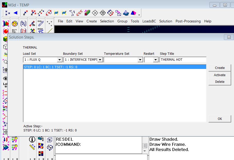
From the drop down boxes select the load-set and boundary-set we created. The restart option is not used. Give the step a meaningful title. Press the "Create" button and then the "Activate" button. In this beta release only the active step is solved. In the final version all steps in the solution will be solved. Press "OK" to exit the dialog box.
Solve
From the menu select "Solution->Solve" this will start the solver and information will be written to the message window.
Plot Temperatures
From the menu select "Post Processing->Select Contour Results" this will invoke the results dialog as illustrated below.
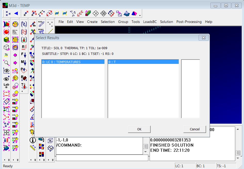
In the dialog select the load-case and the temperature variable and then press the "OK" button.
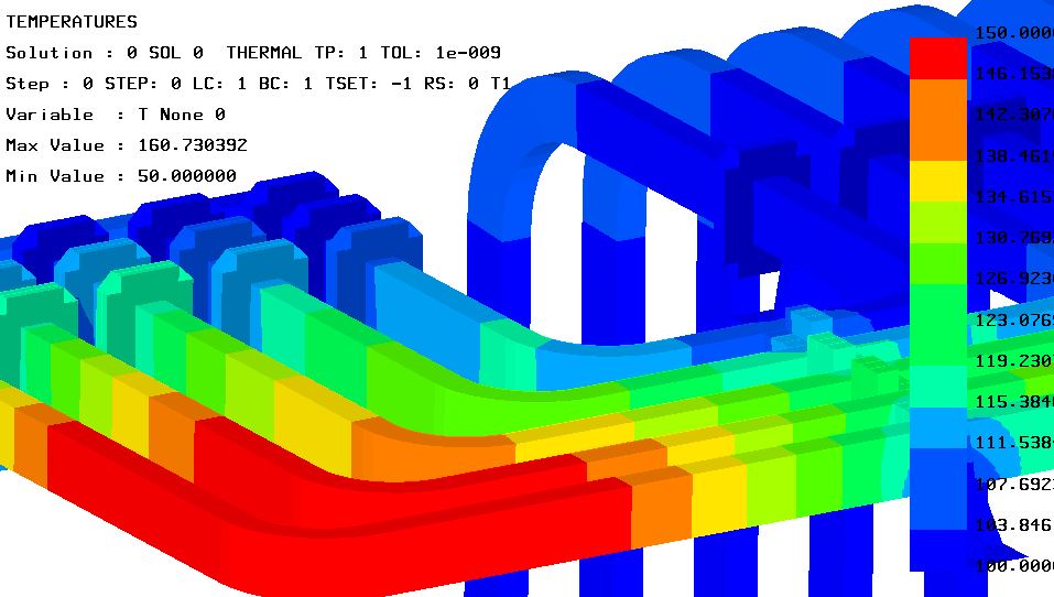
From the menu select "Post Processing->Contour Raw Data" the plot should appear as below.
From the menu select "Post Processing->Contour Raw Data" the plot should appear as below.
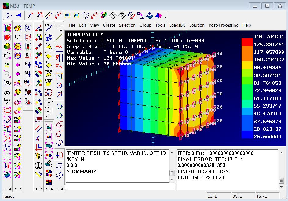
Note that the temperatures will be higher at the edges as we have applied lumped fluxes equally on all nodes. Ideally we need to integrate the flux against the element shape functions in the same way we do for pressures and this will be added.
My hand calculation shows the average temperature should be 36*500/200+20 =110 degrees on the hot end
My hand calculation shows the average temperature should be 36*500/200+20 =110 degrees on the hot end
POST SCRIPT
All the major element types are supported for the thermal analysis, this includes Beams, Shells, Solid and Springs.
For spring elements you have to define the conductive coefficient in the spring property definition. You can use this to create interface contact resistances between solid components. I intend to add convective wall functions and radiant heat exchange (with ray tracing) defined on shell elements.
Comments and suggestions are most welcome, please contribute.